Uncategorized – Verdigris

May 10, 2020May 11, 2020

Simple model examples

Here are some simple model examples. Please feel free to use them, but only subject to the disclaimer that you do so at your own risk, verdigris makes no representations as to their correctness, and takes no responsibility for their use.

Simple debt corkscrew.mortgage style

Simple debt corkscrew.equal principal repayments

Simple property rental model

Sickness decrement model: We put this together for interest to understand what sort of drivers the rate of infections for COVID19 has. The model is extremely sensitive to changes in assumptions (of which there are several). Due to the sensitivity, and to lack of available data for determining the assumptions, it probably doesn’t make a good predictor for infection rates. The influence of a future vaccine is also ignored. If you’re interested, play with the number of contacts per person per day, and the probability of transfer given contact with a sick person. It’s clear from playing with these just how sensitive the infection rate is to very small changes.

April 30, 2020April 30, 2020

Modelling an infrastructure portfolio

Infrastructure investors may over time acquire a portfolio of assets, whether they be equity or debt investors. In South Africa, this is happening in the renewable energy space, with different investors acquiring sizable portfolios of wind and solar projects. Sometimes investments into individual projects may be quite small in comparison to the full portfolio, but the work associated with managing an investment into a project is, unfortunately, not proportional to the size of the investment.

Investors will likely need to value their investments periodically – for example, when they are completing their annual financial statements. They may also need to manage their liquidity, and therefore need to identify what future capital commitments they may have, or debt payments or equity distributions they may receive.

These exercises require a project model for each project in the portfolio. Usually the project model will be the lenders’ base case model (also the bid model in South Africa). As a result the investor will need to maintain several different models, updating each of them for each valuation or exercise. Clearly this becomes more onerous as more projects are added to the portfolio, particularly since each model may have its own idiosyncrasies.

So what steps can such an investor take to simplify the modelling requirements for their portfolio of assets?

I wrote a proof-of-concept portfolio consolidation model recently. Here is the approach I took:

1) Write a generic project model which does away with much of the complexity required for a full bid model and a full bankers’ base case model. In my case, I was looking at operational projects, so I removed construction-period functionality. I also removed all bid-related functionality.

2) Assumptions for the model will be either constant over the full project life (eg name plate capacity), or time-based (eg interest rate curves, CPI curves, debt sculpting). Constant assumptions should be in a single column in the assumptions sheet, which should contain references to the curves applicable to that project. Because assumptions are in a single column, it is possible for the model to include assumptions for multiple projects, each in its own column. I also created a single column for the assumptions which feed through to the active selected case using a lookup to the active project’s assumptions column.

Time-based assumptions, or curves, should be in a separate sheet. I wrote a macro which creates named ranges for each curve item, so that I can then pull a curve into my model dynamically using Excel’s INDIRECT function.

3) The generic project model should be in a single sheet, to the extent possible. By selecting the project in the Assumptions sheet, the calculations will update to represent that project. Given that projects may be structured differently, it may be necessary to have some functionality which is superfluous to some projects, but necessary in others. Examples of this may include multiple debt facilities, a mezzanine facility, O&M bonuses which are structured in a particular fashion, different lease arrangements, and so on. It is necessary that you be able to zero each of these without breaking the model.

4) I created functionality to pull time-based tariffs and balance sheet items into the model. This is because as these change over time, the future distributions to capital providers change too. For example, an increase in tariff (relative to the original base case) will increase the distributions to shareholders. Similarly, a change in the tax depreciation schedule will influence the amount of tax paid in the future and therefore CFADS. It is important that these be included only in the time-based assumptions, and that no changes are made in the calculation sheet, since we will iterate through the projects when working at a portfolio level, and hard-coded figures in the working will clearly break this functionality. You can see an example of these in the Curves sheet in the image above.

5) Now that we have a full project model which is able to represent multiple different project by changing only the assumptions, and the ability to switch between different projects by selecting which set of assumptions to use, it is possible to iterate through the projects using a macro by selecting the relevant project, resolving any circular references, and hard-copying the desired output into a portfolio view for each project. Since each project can have different length and starting-month periods, I used a monthly timeline and a lookup to copy distributions to shareholders (the output I chose for my proof of concept) into a table.

I also created basic error checking, focusing on whether the circular references had been resolved in each iteration, and whether the assumptions in the relevant project were different at the time of running the portfolio consolidation macro to those presently persisting in the model assumptions, using a checksum of the model assumptions.

6) Finally, I aggregated these results into more usable time periods (eg annual), and calculated a range of NPVs.

The approach described here has a few significant advantages:

Most obviously, the investor only has to understand and maintain a single model.
This also means that the single model can be audited at much lower cost than auditing several models.
Implementing scenarios across all projects simultaneously is trivial – for example if the house view on CPI changes, or the VAT rate changes.
Implementing structural layers, such as structurally-subordinated funding, is also fairly trivial.

Overall, these amount to a significant decrease in the amount of time required to perform any function requiring the project model(s), better operational risk management, reduced costs, and to better understanding of the portfolio.

March 21, 2019May 29, 2019

Valuing infrastructure projects

From time to time an infrastructure project or its [potential future] shareholders may need to know the value of the project’s equity. Generally this will be for the purposes of a sale or purchase, or possibly for a listing.

It is most common to use a discounted cash flow methodology when conducting such a valuation. Most of the time this is fairly easy, as the project is likely to have a project model which produces distributions to shareholders at the bottom of the cash flow waterfall.

However, there are a few considerations to take into account when conducting a valuation:

Starting balances

Unless you are conducting the valuation as at financial close, the project will have built up certain actual balances during the construction period and any operations period that has elapsed. These will include the likes of cash in bank, debtors, creditors and plant and equipment. It is best to source these from the most recent set of financial accounts or management accounts available, as these will be the most accurate figures available. These balances will need to be incorporated into the project model such that in due course they feed through to the cash flow waterfall accurately. For example, a debtor balance will, via the model’s working capital assumptions, feed through into the cash flow waterfall and ultimately to distributions.

Starting balances, even cash balances, should not be included as stand-alone sums in the valuation. This is because the timing of distributions creates a material difference to the valuation, and generally any balance lacks this information unless it feeds through the waterfall. For example, a cash balance may result from a debt covenant lock up, which may only be cured in several months’ time.

More information about incorporating balances into the project model is available here: Operationalising Project Models.

Input assumptions

There are three main sources of assumptions available to the valuer:

The Project Documents and the Finance Documents. Good examples of such assumptions are base tariffs prior to inflation and interest margins. These assumptions will, all things being equal, hold for the life of the project, and consequently the valuer should leave them unchanged in the base case project model.

Expert information. Certain technical and macroeconomic assumptions may have been set by experts at the beginning of the project life or subsequently. An example of such would be future fx or inflation assumptions. These are best sourced from a (reputable and justifiable) expert source. Some technical assumptions may not change considerably over the life of the project, and may therefore be left alone without significantly effecting the valuation. An example of this might be power plant capacity.

Note that some project models may have a lenders’ base case and an equity base case. Typically it is most appropriate to use the equity base case (eg P50 energy yield assumptions) since it is the distributions which are being valued.

Actual experience. The performance of the project may differ to the original expected performance, in which case, in the absence of a reason to the contrary, the assumptions should be updated to reflect the most recent experience. Experience should be of reasonable duration – 12 months might be a good starting point to incorporate a reasonable sample size and any seasonality effects. Non-contracted opex inputs are a good example here, as is recent technical performance. Obviously when updating assumptions to reflect recent performance, one needs to apply a reasonability filter. Updating opex or technical assumptions to reflect an abnormally good or bad year will create bias in the valuation. One also needs to ensure that the experience is adjusted to account for the model’s inflation from the base date of the assumptions to the present.

A critical valuation assumption which deserves particular mention is the risk discount rate used to discount the distributions back to the valuation date. There are different means of arriving at, and influences upon, the appropriate discount rate for the valuation, and often some judgement will be required. These may include the following:

If the valuation is part of a sale negotiation, the risk discount rate may have been negotiated in advance, with the monetary valuation flowing from the risk discount rate as a result;
There may be recent sales which provide discount rate market benchmarks;
The project may have been structured so as to arrive at a reasonable risk discount rate for the risk profile of the project, as at the date of development;
The project may have experienced certain milestones and events which increase or decrease risk. An obvious one of these is the project completing construction and reaching Commercial Operation Date successfully. Another is the acquisition of an operating track record of a statistically significant sample length;
For completeness, there are theoretical models for determining an appropriate risk discount rate using the market risk free rate and the project’s beta and leverage – the Capital Asset Pricing Model (CAPM). Such a model is perhaps less relevant for an infrastructure project than for a normal operating company.

If a particular assumption has considerable uncertainty and has a significant effect on the distributions of the project – eg if plant output is very uncertain in the future for some reason – then it may make sense to model that assumption into the project’s future explicitly, rather than by modifying the risk discount rate to reflect the additional uncertainty. This allows greater understanding of the change in the valuation resulting from poor performance relating to the assumption in question. A good example of an assumption like this may be the traffic experience in a toll road project.

Valuation date

The date of the valuation may have considerable impact upon the valuation. In particular, moving the valuation date later by a month will have the following effect:

The valuation will increase by approximately 1/12^th of the discount rate; and
The valuation will decrease by any distribution that was in the valuation period before the date change, but is no longer in the date change.

Consequently, if distributions are semi-annual, the valuation can move as much as 41% of the discount rate from a 5-month change in valuation date.

Termination amount

If one simply discounts the distributions in the project model, it is possible to miss the residual value of the project at the end of the project term (usually the end of the offtake contract term). This may be completely appropriate, for example in the case of a Build Own Operate Transfer project. However, in other instances it may not be appropriate at all, such as in the case where it may be feasible to enter into another subsequent offtake contract, or dispose of some of the project’s assets for a sum. Conversely, a rehabilitation cost may be applicable at the end of the term. Such an amount may be modeled explicitly by discounting the sales price or rehabilitation cost, or by extending the term of the modeled operations period using a new set of (possibly conservative) assumptions.

Sensitivities

The valuer may be asked to provide a single valuation figure, but it is nonetheless good practice to provide sensitivities to those assumptions which either:

Have considerable uncertainty;
To which the valuation outcome is very sensitive; or
Both.

The purpose of the sensitivities is to help the client in any final negotiations or decisions around the final price or valuation. If the final report is a public document, or shared with the other side of the negotiating table, these sensitivities could be removed from the final public version of the valuation report.

January 23, 2019May 29, 2019

Operationalising project models

Why do it?

Once a project has been through its financing and construction phases, the project may want to operationalise the project model. This can have the following benefits for the project:

The model can be simplified, making it more tractable to use, since much of the financing-related functionality is no longer necessary;
The construction period can be removed, further simplifying the model;
We can incorporate actual experience, making the stepping-off point for projections much more valid than under the original base case model;
We can integrate the model into the project’s existing administration systems; and
We can incorporate new line items which were not considered relevant at the financing stage – in particular, new opex items are common.

Operationalising a model may be more important for a project if the project’s reality has evolved in a fashion which is significantly different to that portrayed by the original model. Such an eventuality may necessitate frequent reconciliations between model and accounts, explanations of budgets and justification of covenant ratios.

Starting point

The inputs required to operationalise a model include the following, assuming the modeler has some familiarity with the project:

The original model;
At least two sets of financial statements and/or management accounts (or general ledger and mappings from the ledger to the fields in the model);
An indication of what new functionality is desired, if any;
An indication of how frequently the project would like to incorporate actuals into the model, in order to determine the period of the new model.

I recommend that the modeler start afresh or use a template for the new model, rather than trying to modify or simplify the existing model. This is because simplifying an existing model comes with any baggage associated with that model, and it can therefore be cumbersome. A simplified model may end up with inputs and calculations with no dependents, and may incorporate logic errors which were overlooked in the original model build.

Process

I recommend splitting the process into three main sections:

Stage 1: Replication and simplification

Replicate the existing model in a simplified manner. There will be much functionality which is no longer required, such as being able to select between different facility types (eg mortgage-style vs equal principal repayments). In this example the project has now fully determined which is applicable, so abandon the other. Another example may be excess facilities penciled in in case they were required, or construction period functionality.

Having the original model available is very helpful in understanding what the mechanics are for the transaction, and also to check numbers against. In particular, numbers which are point-in-time (such as revenue received in a period) as opposed to cumulative (such as cash balance) are ideal to check against the original model at this stage. I tend to check these as I work through the model build, and colour code my checked values to easily see which are exactly the same as the original model, which are similar, and which differ. Doing this will also help model users (lenders, for example) reconcile the new model back to the original model. This is helpful because it’s very likely that they made themselves comfortable with the original model, which was probably audited. It will also assist with model audit, if such is required.

Stage 2: Incorporating actuals

I like to incorporate a full new sheet which only contains actuals (i.e. figures that have actually occurred, and can therefore be found under existing sources of macroeconomic data (eg inflation) or in the project’s financial statements or general ledger). The benefits of this are:

That the project / model users do not have to search through all your calculations to determine where to fill in their actuals;
This in turn means that there is a reduced possibility of modifying the model’s calculations and thereby breaking it;
Actuals are all in one place, and can be located with appropriate mappings so that new line items can be more easily incorporated into the model in the future. It should therefore also be evident if one or more actuals are omitted.

Actuals on a single sheet, incorporating mapping information

Depending on what the client wants, the actuals to include may be a full dump of the management accounts, general ledger or financial statements, or a subset of that information. Since the project will be updating this sheet periodically, it needs to be clear what each actuals line item incorporates, and how that information is to be sourced in subsequent periods.

If a subset of the management accounts is acceptable, it’s usually sufficient to use a combination of balance sheet and income statement items. Cash flow statement items can typically be implied from these.

As implied above, the actuals sheet may also include a series of mappings. This is because the model is likely to have less detail, aggregating several rows from the AFS or general ledger into fewer lines. The mappings, in conjunction with a SUMIF function, can effect this.

From the Actuals sheet, I typically import the aggregated/mapped rows straight into the top of my Working (i.e. main calculations) sheet. These then feed down into the model’s projection calculations using a formula similar to the following: =IF(actual <> “”, actual, projection). You may also need to infer certain revenue items or expenses from the balance sheet items which you import. This is necessary to minimize the size of any balancing items. I also tend to place conditional formatting in my worksheet to indicate where the figure observed has been pulled through from actuals, or is a projected figure.

Conditionally-formatted actuals pulling into the Working sheet

Finally, one or two balancing figures will probably be required. If you import actual cash balance at the end of the period, it is unlikely that the cash flow waterfall will balance, since some items will be projections/ calculated values and some will be actuals. A balancing cash flow is therefore required to reconcile the starting balance and sum of all cash flows in the period with the ending balance. This balancing cash flow should automatically be zero in periods which have no actuals being pulled through. Obviously this should be as small as possible. Another balancing figure may be required to reconcile starting balance sheet figures plus income statement items with the actual end-of-period balance sheet position. Again, this should be as small as possible. However, note that this balancing figure will persist (without changing, otherwise something is wrong with your model) into projected periods.

Stage 3: Importing actuals

Finally, you should import at least two periods’ worth of actuals into your model. This will ‘settle’ the figures, since the first period sets the base line, and the second period creates the first accurate set of the implied / calculated values which result from the previous accumulated position and the present period’s actuals.

As a corollary, many of the calculated figures in the first period may be incorrect / spurious. This is because the model is moving from one basis (projections) to another (actuals). Any accumulated values (such as cash balance) may differ significantly between the two bases.

A second advantage of incorporating multiple sets of actuals into the model is that it will provide a better base for model users to compare against when they first need to incorporate actuals without the benefit of having the modeler present to assist.

Amount of work required

Operationalising a model is significantly less work than building a project model in the first instance. This is not so much because there is less functionality (although that may be partially true if the new model is much simpler than the old model), but because there are fewer moving parts to the project itself, and because the old model provides as good a set of assumptions and inputs as a modeler is likely to receive.

May 19, 2018May 29, 2019

Framework for writing a trading algorithm

I’ve been lucky enough to have some spare time to look at projects of my own this year, so I researched and implemented a number of trading algorithms on various crypto currency exchanges.

Investing vs trading:

Before we start, though, a quick disclaimer: I’m undecided on the merits of crypto currency as an asset class. My intention here was to implement one or more algorithms to hunt arbitrage opportunities and, upon finding them, make the trades that would implement them. Where I have taken exposure to crypto currencies, I have both won and lost. Consequently, I don’t consider myself to be invested in crypto currencies, as I can’t foretell the future of the asset class with sufficient certainty for my somewhat risk-averse predilections. I’m happy to trade it, though – particularly if I can do so in a manner which minimises my exposure.

Why crypto currencies, not traditional exchanges:

For me there are three reasons which made crypto currencies a good learning ground for this sort of exercise:

It’s generally accepted that the crypto currency markets are fairly inefficient, meaning that arbitrage opportunities abound. This may be because the asset class (without discussing the merits of such a label) is in its relative infancy, and it may also be because there are a large number of new, as-yet relatively unexplored exchanges.
Crypto currencies are extremely volatile, which means they’re likely to move faster and further than traditional asset classes. Arbitrage is based on the differentials between prices or returns on (typically correlated) assets. More movement means a greater frequency of those differentials occurring.
Crypto currency exchanges are created by IT people, and their APIs (Application Programming Interfaces) are fairly unrestricted. I’m not sure about all traditional exchanges, but as an example, the JSE does a full code review of any code which hooks into their exchange. The wild-west of crypto exchanges don’t. It’s also pretty cheap to register and start trading – no monthly stock broker’s fees, etc.

Where to start:

There are two possible places I can see to start with creating a trading algorithm (or algo). These are:

The theoretical framework for the trade; and
Collating the data.

Theoretical framework:

I did a lot of reading about different types of arbitrages to determine what might be suitable. In reality, I suspect that just about any trade which exists in a given traditional market could be implemented in a different market (whether traditional or not).

The more complex the theoretical framework for the trade you want to look at, the greater the difficulty in implementing it, and the possibility that it could go wrong. On the other hand, complex trades are likely to be less prolific than trades which are simpler or more vanilla.

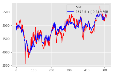
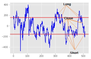
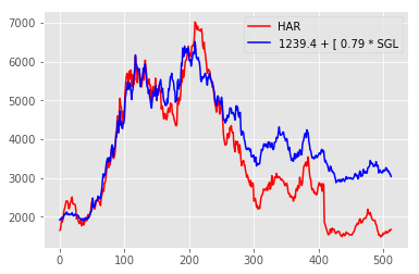
The sort of behaviour we’re looking for is [statistical] predictability. This could be in the form of correlation of leading and lagging indicators, it could be a stationary process, it could be misaligned prices, mean reversion, momentum, or, for that matter, anything else which you hypothesize may give you an edge.

The common element in all of the above is that we want to have a better than 50:50 chance of predicting the next move in the price of whatever it is that we’re trading. Sometimes that behaviour is statistical in nature, such as stationary processes (used in pairs trading, for example) and sometimes it’s more simply a function of efficiency in markets, such as misaligned prices.

Collecting data:

You can almost always find relatively clean data to purchase, if you wish to go that route. It has many advantages: It’s easier, possibly cleaner and almost certainly has a better (longer) history than you could get yourself. On the downside, you’re spending your seed capital which you could have used for trading instead! Also, you don’t necessarily have oversight on how the provider has cleaned the data, and the granularity may be incorrect for your purposes.

If you choose instead to collect your own data, bear in mind that historical data may not be easily available, or available at all. This means you might want to start collecting as early on in the process as possible, so that you have something against which to test your trading hypotheses.

I chose to collect my own data. If you’re looking for historical data for traditional markets, you can download dumps from various sources, such as google finance (stocks, currencies), xe.com (currencies), various reserve banks, etc… For traditional markets, I found that this was helpful in trying to understand the data better, but not particularly helpful in testing trading hypotheses. This was almost all down to the lack of granularity of data available for free. However, I understand that traditional market data is available at fine granularity through the likes of Reuters, Bloomberg and other such providers – but read up on how they collect and clean it!

On the crypto currency exchanges, I hooked into multiple exchanges using their APIs and downloaded order book information for relevant instruments (currency pairs, underlying vs future vs option) at a granularity of around a minute, typically. My little downloading app runs on my pc pretty much 24-7, pulling data from a dozen exchanges each minute. I also collect fx data by screen scraping, although I have run into occasional rate limit issues, which seems fair enough to me, albeit it’s frustrating when it happens.

When I first started looking at crypto currencies I found an excellent project on github called ccxt, which is an open source integration into, at time of writing, 115 different crypto exchanges. This allowed me to do a very quick and dirty download of tick data to try and find correlations and misalignment between different exchanges, instruments etc. I used python (anaconda / Jupyter notebooks) for this exercise and stored my data in a Microsoft SQL Server database. (Both of these are free downloads, although there are some limitations on free SQL Server.)

What data to fetch:

If you haven’t decided exactly trade you’re going to implement, and therefore don’t have sight of your specific data requirements, I recommend fetching per-minute tick data from an assortment of exchanges which may be relevant to you (because you think they’re safe, the instruments being traded are of interest, the geographies work and the volume and liquidity on the exchange is sufficient for your purposes, for example). Collect data for instruments which are of interest – rather too much than too little, since you can always delete it, but can’t go back and collect it again. Initially I started collecting the market ticker information, but I abandoned that fairly soon in favour of only order book data – or at least the top several levels. I currently fetch ten order book levels, although that may be overkill, since I’ve yet to actually use anything other than the top level of the book. As mentioned above, I also collect the fiat fx rate for each order book fetch which has a fiat side (eg USD-BTC) back to a common currency. As I’m based in South Africa, that was ZAR, but you should use whatever works for you, obviously. Given that you’ll be making dozen’s of order book fetches every minute, I recommend storing the fiat fx rate locally periodically and referencing that (or pay for a service provider that doesn’t mind you hammering their server).

You’ll probably also want to fetch any underlying for any derivative instruments you’re collating information on – such as the index for a futures contract.

Finally, I recommend multi-threading your data collection. Although it’s more complex than a single-threaded application, this allows the time differential between data fetches on different exchanges to be smaller. By way of example, a single-threaded application might fetch data at 10:00:00 on exchange A, 10:00:05 on exchange B…. 10:00:30 on exchange Z. If you want to identify price misalignment between exchange A and Z, you will not know what portion of any misalignment you identify results from differences between the exchanges, and what results from change in the underlying price between 10:00:00 and 10:00:30.

Admittedly, you could be a bit obsessive about this. Spurious Accuracy and all of that…

Hypothesis testing:

We now have a gross hypothesis, and the data to test it. So how do we go about doing so?

In the simplest form, we need to simulate the trade we wish to do. However, a trade will be dependent upon some detailed assumptions and decisions (i.e. parameters). We should therefore find and test these parameters. This is something of an iterative process.

Parameterisation:

Firstly, what sort of parameters are we envisaging here? Examples that come to mind include:

The period of the data we’re looking at to determine the behaviour of the next tick (Last month’s worth? Last hour’s?)
The granularity of the data (minute, hour, day, second, microsecond)?
The underlying instruments we’ll be trading (base token (which currency pair?), future (which strike date?), option (put, call?))
The exchanges we’ll be looking at
The measures we’ll be using (standard deviation, correlation coefficients, mean return, direction, SMA, EWMA… many many to chose from)

There will be a number of different ways to determine and optimise the parameters for our trade. Remember that we’re looking for predictive relationships, which implies that correlation (or covariance) is a great place to start. If that’s a starting point you’d like to try, then you want to sort your data into leading indicators (input data) and lagging variables (the subject of your investigation). I found Anaconda python, numpy and SciKit Learn to be fantastic tools for this (A quick aside: I am constantly amazed and gratified by the number of super-clever people out there who create these tools and then make them available to everyone for no cost!). I found that identifying the covariance between leading and lagging indicators was a good starting point and then testing whether than might translate into a trade using simple regression worked pretty well for me.

A few points about this stage of the process: I found several warning references in literature regarding overfitting. I did try out various machine learning frameworks (Keras and Tensorflow’s neural networks and recurrent neural networks, for example.) However, I eventually abandoned them in favour of simpler methods. I’m not saying that I won’t go back to them, but it felt a bit like smashing a nut with a sledge hammer – the tools may have been a bit overpowered for what I wanted to do, and I was not able to predict the problems that might arise – which clearly you want to avoid if there’s real money on the line.

Simulating the trade (or “backtesting”):

Having identified a starting set of parameters, the next stage is to simulate the trade. You can do this with various levels of cleanliness, and it’s good practice to start dirty and then clean up if the trade looks like it might work.

Given we’re trying to implement an algo, your simulation should look something like this:

Start loop through time (t):

—If some condition exists:

——Execute trade 1

—If another condition exists:

——Execute trade 2

…etc…

Move to next time step

Initially, I recommend that you don’t bother with fees, volumes, lag times for hitting the exchange, etc – just see if the decisions that you make to trade result in a profit or loss, and what the variability of that profit or loss is. If you make a profit, but first lost more than your capital, then the trade may be too risky to implement. You can also use risk-adjusted return measures, such as a Sharpe Ratio, to measure the success of your trade. Ideally you want a profit curve that slopes consistently upwards, with any downward swings being limited in size (obvious, I know!) My point is that certain trades may be very profitable, but just too risky – I abandoned a number of trades which are more profitable than the ones I landed up implementing because of this.

You also want to watch out for spurious profits – eg, if my algo was simply a decision to buy BTC under any circumstances, and I backtested my decision to buy BTC over 2017, my algo would have looked immensely successful. If I had then implemented it in live in 2018, I would have been crushed.

Once you have done your simple back test, and if the results are encouraging, you should increase the detail of the back test. In particular, you should implement the fees. Other things to look at include:

The amount of collateral or margin you’re using relative to your available limits – you should limit your maximum position such that the probability that your margin requirement increases above your available margin is below an acceptable probability;
The volume available at the prices that trigger your decisions to trade – if there’s almost no volume available at those prices, then no matter how high the return of your trade, the trade won’t be able to execute sufficiently to justify the time spent in coding it;
Lag times for hitting the exchange – if you are not going to be able to hit the exchange with zero lag upon the conditions for trading becoming true, what is the impact of the delay?

Tools for backtesting:

I like two (or maybe three) different tools for backtesting.

I mentioned above that I use SQL Server to store my data. I also use it to create the data dump which I will simulate my trade on. SQL allows me to slice, dice and order the data, build simple comparisons or functions on the data, and to exclude anomalous data. It’s not ideal for detailed loops, though…
Python: Python has lots of libraries which assist in financial data analysis (like Numpy). If you’re not au fait with any particular tool, and are going to have to learn one to get started, you could do a whole lot worse than Python for this. Python also allows you to save your data in pickles, so you don’t need a database at all, if that’s what works for you.
Excel and VBA: I discussed using Excel and VBA for my backtesting with a family member who is an algorythmic trading programmer, and was nearly laughed out of the room. (Thanks Steve!) However, there are a few things which Excel has to recommend for itself. I feel that the familiarity of the environment helps you get started quickly, although you will very likely need VBA, so this may be moot if you’re not familiar with it. Not that you can’t do the same with Python, but I also liked creating functions which put out the result of my simulations, and then calling them from tables which laid out the profit with different combinations of input parameters to create a heat map with conditional formatting (which you can also do in Python, now that I think about it).

Python is much quicker at crunching this sort of data than Excel, for a given quality of code.

Fine tuning parameters:

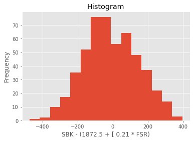
I like to create visual representations of my outputs so I can home in on success and risk easily. Heat maps are good for this.

Here’s an example:

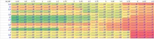
The heat map tells us where there are (relatively) successful combinations of input parameters (halfway down on the left) vs unsuccessful (on the right). When choosing parameters based on the heat map, you ideally want to choose a parameter which is not only optimal, but also surrounded by good outcomes. Should the true underlying conditions of the trade change slightly, this should maximise the chances that the outcome will still be relatively optimal. Consequently, in the above map, I would posit that an outcome in the center of the green would be better than a (hypothetical) outcome with an even better profit surrounded by red (i.e. poor) outcomes. The particular algo I was looking at in this example has 6 or so parameters, while clearly you can only (easily) represent two in the heat map. That’s okay – ideally your algo should have local profit maxima with respect to each parameter which are relatively independent of the other parameters. If not, you run the risk that interactions between your parameters may create risk which you don’t understand and cause your algo to lose money. Test this by creating multiple heat maps for parameters outside of the table and seeing if the profit transitions from one table to another in a relatively smooth fashion.

I touched on the dangers of overfitting above very briefly. I don’t think that optimising parameters constitutes overfitting, if you have already chosen your algorithm. However, remain vigilant, particularly if your algo is complex and requires many parameters. (If it is, go and read up on overfitting!)

A second output of my analysis is always a tick-by-tick graph of the profit, showing when trades occurred, what my open position is (to track margin requirements if I’m looking at derivatives), and my current balance (PnL). I usually only create this for trade/parameter sets which are successful / optimal, since I’m not interested in the others anyway. This allows me to identify the track my algo took to get to the optimal outcome. As I mentioned earlier, if I had to lose $1000 first in order to eventually make $100, then the algo is extremely risky relative to the outcome, and probably not worth implementing.

Implementation:

Right, so we’ve now identified a likely-looking trade and we’re ready to implement it.

I initially tried to write a generic framework which I could parameterise to implement any algo. Although this had some success, I became worried that it added more complexity than it was worth – leading to higher latency and greater possibility of error.

I settled on an intermediate approach. I write relatively generic ‘ExchangeMethods’ which hide the complexity of actual interactions with each exchange, but look similar to the rest of my code. Examples of my exchange methods include:

Market Order
Limit Order
Get top price and volume
Cancel order
Get open position from exchange
Get open orders on exchange
Get collateral balances on exchange

I then write the algo execution code (this will look similar to our pseudo code above) which:

Fetches the [order] data from the exchange

Checks to see if the conditions for opening or closing a position are now true

If so, implements the trades which will open/close the position

loops back to the top and repeats indefinitely

In theory, if I want to use a different exchange or instrument, I can then simply swap out the parameters for my ExchangeMethods and off we go. This is not quite true in practice, but I have managed to implement similar algos to pre-existing ones on new exchanges in under a day, so there is some merit in the approach.

I chose to use C# for my implementation, as I had some pre-existing familiarity with .Net, if not C# itself. However, I would suggest that Python or Java would have been better, because they seem to be more popular, with the result that more of the example code for connecting to different exchanges exists in those languages than C#. For obvious reasons, this can reduce your time-to-delivery for writing exchange methods. I have, however, found C# to be perfectly adequate. It has plenty of literature available, and does everything I need of it. I also like the slightly more structured environment (SDE).

As with data collection, I recommend multi-threading your exchange methods. This allows multiple trades to be placed in the order book at the same time, which may be important if:

We are trying to trade only when the conditions which trigger our trade are true – they may have changed if we delay our trades; and
Perhaps even more importantly, if our trade conditions relate to a (possibly calculated) differential between the prices of two or more different instruments. We wouldn’t want to trade one at the ‘correct’ price, but not the other.

I recommend putting a lot of logging into your code, and particularly into your Exchange Methods. This will help you with debugging, and also with determining why your trade is successful or not. Log each decision you’re about to make, and the outcome. Log (nearly) every interaction you make with the exchange (I maxed out by database size logging 100 price fetches per second – hence the ‘nearly’). Log the conditions that apply when you trade, and log the prices and volumes you think you’re making a trade at (the “trigger price”). Some exchanges allow you to place a user-defined data item into your orders. I recommend filling this with, for example, the trigger price, volume, your open position, your collateral balance and a short but meaningful metric which describes why you’ve made the trade. In due course, you should then be able to download your trades and use the custom data item to show how successful you have been in executing at the conditions you thought prevailed. An obvious example: If your trigger price on a buy market order is 1% higher than the price which you actually bought at, then your execution code is probably too slow.

Is exchange microstructure an issue?

Unequivocally…hell yes.

Different exchanges have different microstructures. These are seldom (never?) documented, let alone well documented. They can wreak havoc upon your best code and intentions. Unfortunately determining what the microstructure is seems to be an almost entirely empirical process. I consequently recommend that you start with only a small balance on any given exchange and trade that for a while. I have been caught out by microstructures, lost money because of them, and abandoned algos that looked promising because of problematic microstructures. They waste time and energy (coding for exceptions / unexpected exchange behaviour is difficult!). If you can, read up as much as you can about an exchange before trading on it. If there are lots of questions from confused algo traders… maybe it’s significant!

Another topic which relates to microstructure (sort of) is latency. It may not be clear where your exchange is hosted. If your algo requires low latency, you may want to do some research on this. Hosting your algo in the cloud in specific geographic locations may be helpful – you can test this empirically. I haven’t yet reached the stage where latency is an issue for me, but there is some literature / discussion online about this sort of issue.

Other things to look into:

Without going into too much detail, I suggest the following things are worth looking out for / understanding more of in the context of your trades:

Margining calculations – I’ve been caught out by this one
Balancing of equity (collateral) positions, particularly between different exchanges if you’re implementing a trade across more than one exchange – Caught out by this too
(Unrestricted) ability to withdraw equity – And this
So-called “Socialised Losses” and Insurance Funds (but not this…yet)
Rate limits – I’ve had to create lots of extra code to get around rate limits
FEES! Actually, big fees are as much of an opportunity as a hindrance, since they almost inevitably result in greater differentials
Leverage

Some metrics:

Time spent on this project: 5 months, nearly full time

Exchanges integrated into: 5 for trading, ~double for data feeds

Algos that worked on paper (or in Excel!) but not on the exchange: Far too many.

Passing shot: Pavlov’s dog

I set a system chime to sound every time my algo traded, which it duly did. However, I initially used the generic Windows system exclamation sound. Which was fine for a while, until I found myself charging off to have a look at my screen every time my wife made an illegal key entry on her laptop. I recommend using a non-standard chime.

If you have any questions about any of the above, please feel free to contact me – contact details elsewhere on the site.

November 11, 2017May 29, 2019

Exercise on stock pair selection using South African data

The premise for the long/short stock pair arbitrage trade

The long/short stock pair trade is a well-known arbitrage trade, which works as follows:

Identify two highly-correlated and co-integrated stocks.
Establish that each stock and the long-short combination of the two stocks is indeed stationary. Steps 1 and 2 are referred to as the Engle and Granger procedure.
When the two stocks move away from each other, short the stock that has increased in value and go long on the stock that has decreased in value.
Since the two stocks are highly correlated, they should move back towards each other at some point, closing the gap between them.
When they do, close out the positions. At this point, the aggregate value of the long/short pair should be greater than zero, since in order for the gap to have closed, the shorted stock should have decreased in value relative to the value of the long stock (or visa versa).
Since this is a statistical arbitrage strategy, repeat this exercise over as many pairs as is reasonable in order to reduce the possibility of a (hopefully!) low-probability event that the correlation observed to date is simply a statistical fluke which does not continue into the future.

If the premise upon which the trade is based is correct, and the correlated stocks are chosen appropriately, the portfolio should be profitable.

Building the model

I built a model to test this trade based on the more liquid stocks on the Johannesburg Stock Exchange (JSE). Doing so entailed the following steps:

Obtaining stock data:

I downloaded stock data from google finance using excel and vba macros as laid out by Edward Bodmer in his excellent financial model resource website, https://edbodmer.wikispaces.com. To do so, I looped through a list of JSE stockcodes and used the Workbooks.Open (URL) Excel method, where URL is replaced by the URL of the google finance page for the stock I wanted to download. I pushed all of these values into a SQL Server Express database so I could slice and dice the data later when I needed it. Unfortunately google finance doesn’t do adjusted prices (i.e. prices adjusted for share splits and dividends) so this might be a possible augmentation for a later date.

Testing for stationary time series

I filtered my stock data to ensure I only used liquid stocks. Then I generated a list of stock pairs for every combination of liquid stocks. I did this in SQL, before moving each pair into a Python scripting environment where I tested that the change in price of each stock (i.e. ClosePrice today – ClosePrice yesterday) was stationary. To test that each of these two time series was stationary, I used the Augmented Dickey Fuller test, which is available in the statsmodels python module. I used a 95% probability threshold in my test, rejecting any stocks or pairs which were not stationary with probability of at least 95%. These tests were undertaken on roughly a year’s worth of data (October 2015 – October 2016).

Checking for correlation and co-integration

I randomly split the data for for those stocks which had passed the stationarity test (stationarity is actually a real word!) into an 80% training population and a 20% testing population and used this to conduct a regression on the stock pair, with one stock being the input (x) value and the other the output (y) value. Again, I used python, using the LinearRegression model in sklearn. I validated the regression using the remaining 20% of the data, saving the accuracy score and the regression coefficients. For example, SBK = 1872.5c + 0.21 * FSR. (A Standard Bank share will cost you roughly R18.72 + 21% of the price of a FirstRand share).

I then generated the modelled prices for the output (y) stock using the data for the training year, subtracted that from the price of the input stock (x) (there’s the long and the short!), and tested the difference for stationarity. If it wasn’t stationary, then, assuming the premise for the pairs trade holds, we couldn’t expect the pair to revert towards each other after they move apart. If it was stationary, then a histogram of the values of the long-short pair (ie the difference) should be approximately normally distributed.

At this point, I had a list of stock pairs that passed the three stationarity tests, a set of regression coefficients describing their relationship, and a measure of how well the regression worked (the accuracy score). I also calculated the standard deviation of the long-short pair, for later use.

I ordered my list of pairs by the regression accuracy, moved my data on a year, and simulated a set of trades.

Simulating trades

To simulate the trades, I started at the beginning of my new year and examined the price of the long-short pair (SBK – [1872.5c + 0.21 * FSR] for my example pair above) for each day moving into the future. If the stocks were perfectly correlated, then they would never move apart and the long-short price would remain at zero. If however, in keeping with the trade’s premise, the shares started to deviate in price (hopefully temporarily!) then the long-short price would move up or down.

Correlation graph between SBK and FSR: The first half of the graph shows the period over which the correlation model was trained, and consequently fits really well. The second half is the ‘testing’ period, which shows how well the correlation continues into the future.

I chose the following four rules to generate trades for each stock pair (using our SBK-FSR pair as an example):

Start with a notional cash balance of, say R100,000 (notional because we’re going both long and short… and because it’s fictitious at this point!)
If the long-short price is above 1 standard deviation, and we’re not already long FSR, then SBK’s price has moved up a lot relative to FSR, so go long on FSR and short on SBK. Go long/short the same amount of R100,000, or whatever balance we have if this isn’t the very first trade.
If the long-short price is below 0.3 standard deviations and we’re long, then close out the long/short positions. (I.e. move to cash; add the profit or loss to the new notional cash balance)
If the long-short price is below -1 standard deviation,s and we’re not already short FSR, then SBK’s price has moved down a lot relative to FSR, so go short on FSR and long on SBK. Go long/short the same amount of R100,000, or whatever balance we have if this isn’t the very first trade.
If the long-short price is above 0.3 standard deviations and we’re short, then close out the long/short positions. (I.e. move to cash; add the profit or loss to the new notional cash balance)

A graph of the daily value of the SBK-FSR long short pair (blue) and a single standard deviation of the values (red). The different trades are indicated by the orange lines: Long = 2 above, Short = 4 and Close = 3 and 5. Recall that trading only starts mid way through the graph.

Repeat this across the full year, and for all the stock pairs.

Finally, check the portfolio value relative to the money put in at the beginning.

Did it work?

I got mixed results. If all the pairs had behaved like the SBK-FSR pair then the trade would have done very nicely. However, they didn’t. Here’re the graphs for the Sibanye Gold, Harmony Gold pair:

At the start of the trading period (around day 250) this pair looked very feasible. The graphs correlate nicely over the training period and the big swing and reverse around day 180 looks enticing! So let’s trade…

For this pair, we would have shorted Sibanye and bought Harmony around day 260… and we would have continued to hold Sibanye until the end of the trading period, by which time we would be about 10% down, excluding trading and holding costs.

I see your model and I raise you reality

But why? The correlation looked great, and the trade looked so promising. Simply put, circumstances trumped the correlation:

Google search for Sibanye Gold, limited to the last year (and this is the one we shorted!). Harmony Gold’s looks pretty bad too, with illegal mining, strikes, deaths at the mine and managers being murdered.

Consequently, it looks like you need to be a little bit lucky, or apply a little more than statistical determinants to choosing your stock pairs. This is in agreement with the literature, which speaks to “selecting stocks which have a reason to be correlated”. I.e some judgement is required. It also makes sense in a South African context, since our economy feels fragile and prone to shocks right now.

Consequently, an exercise like the one above might be a good starting point for building a pairs trade, but requires both judgement and quite a bit of model tuning.

Afterthoughts:

Any comments or questions are very welcome.

I can think of quite a few model improvements, amongst them:

A rolling evaluation over the trading period, using data that is in the past, as at the date of trade (rather than a year stale by the end of the trading period)
Stop losses
Inclusion of fundamental economic inputs to identify possible reasons for changes in the correlation
Portfolio constraints, such as exposure limits
Incorporating price adjustments for stock splits and dividends
Use of more granular data

February 26, 2018May 29, 2019

Is volatility in a renewable energy yield assessment good or bad for lenders?

BAD! Or, at least, that’s the general view. As always, however, there isn’t a simple answer.

I once made a casual statement that volatility on a renewable energy yield assessment for a debt transaction I was working on was beneficial from a creditworthiness perspective. My client at the time (the lender) was adamantly opposed to the statement. Since it’s generally the case that greater volatility is bad for a transaction, (and the client is always correct!), let’s look at why it’s bad.

Project finance is, inter alia, lending a principal sum against a set of predictable cash flows. Greater volatility of yield implies less predictability and therefore greater risk of being unable to meet payments when they fall due. This means higher probability of default, higher pricing, less debt-bearing capacity and so on. So volatility is generally bad for a transaction, and perhaps especially so for equity, since debt will only ever lend up to a level of risk which it is comfortable with (one assumes!).

On the other hand, there’s the concept of Upside Risk (https://en.wikipedia.org/wiki/Upside_risk). This is the possibility of a gain in the value of an investment. All other things being equal, the greater the (statistical) downside risk in an investment, the greater the (statistical) upside risk. Upside risk is also applicable to a yield assessment, since it is, after all, a statistical assessment.

Moreover, lenders will usually lend up to a maximum amount limited by the P90 yield assessment. (and the debt:equity ratio, debt service cover ratio levels and other metrics imposed by their credit committees). Assuming the yield assessment is reasonable in determining the P50 yield and the standard deviation of the yield, and that a Normal distribution is a reasonable approximation of the actual random distribution of the yield, it’s helpful to examine the downside and upside scenarios in terms of conditional probabilities (https://en.wikipedia.org/wiki/Conditional_probability, for those of you who like numbers!):

Downside scenario: All other things being equal, the expected yield given the actual yield is less than the P90 level will be lower for a plant with a higher-volatility energy yield than for the same plant with a lower-volatility energy yield.

Obviously when considering such a scenario, lenders would like a lower volatility energy yield assessment, so as to limit possible downside scenarios to a smaller loss (or failure to repay).

Upside scenario: All other things being equal, the expected yield given the actual yield is greater than the P90 level will be higher for a plant with a higher-volatility energy yield than for the same plant with a lower-volatility energy yield.

In this scenario, higher-volatility implies greater CFADS.

Consequently, it is reasonable to balance the risks and benefits of the two scenarios. Under the downside scenario, the risk is that the yield may be insufficient to ensure debt service, particularly if the cover ratios under the P90 base case were tight to begin with. It is worth noting that (assuming the correctness of the yield assessment) this risk has less than a 10% probability of arising (because we’re using a P90, the base case cover ratios being > 1.0x and because Normal distributions with the standard deviations typical of renewable energy projects are relatively long-tailed).

The upside scenario, on the other hand, encompasses 90% of predicted years’ energy outcomes, assuming we’re using a 1-year P90. This in turn means that the CFADS will be larger than under the P90 base case in most years, and, simply, cash can be used to mitigate many risks. The nature of those risks is, of course, very much dependent on how well they are mitigated through the contractual protections built into the project documents. If all risks other than yield are 100% contracted away to the project’s reliable and creditworthy counterparties, then the protection offered by additional cash is worth less than if only a portion of that risk is dealt with. Similarly, if DSCRs are very healthy using the P90 cash flows, the marginal benefit of yet more cash is smaller.

The question then becomes one of whether the benefit of additional cash in (probably) nine out of ten years to mitigate risks which may arise in those years, is greater than the risk of a greater expected underperformance in the one (probably!) year in ten when yield is lower than the P90 level. This is a slightly more difficult evaluation than an all-encompassing perspective that volatility is bad. However, it also offers benefits which may be proposed to a credit committee, for those transactors with a higher-volatility project!

September 28, 2017May 29, 2019

Renewable energy yield analysis

The energy yield assessment is a fundamental requirement for any new wind or solar project, with both developers and lenders spending considerable time with their respective advisers to understand the underlying wind or solar regime. The remainder of this article speaks predominantly to wind energy yield assessment, but the same principles can be applied to solar projects.

Before we start, a short discussion around P50 and P90: The P50 energy yield estimate is the estimate of the energy yield which the energy yield modeller estimates will be exceeded with a 50% probability. Similarly, the P90 energy yield estimate is the estimate of the energy yield which the energy yield modeller estimates will be exceeded with a 90% probability. Consequently, the P90 estimate is lower than the P50 estimate. Although P-levels are usually quoted as annualised figures, the application periods can differ: Hence you may see reference to a 1-year P90 or a 10-year P90. This is simply the estimate of the amount of energy which the modeller estimates will be exceeded in a 1-year period or a 10-year period (multiplied by 10, since it is an annualised figure). They differ because the P90 is a function of the median energy yield estimate and the standard deviation of the energy yield estimate. In the case of the 10-year P90, the uncertainty associated with the estimate is spread over 10 years, so that a bad year can be offset by a good year within the period; or statistically speaking, a larger sample size reduces the variance associated with the estimate. As an aside, because the P50 is simply the median of the probability distribution and takes no account of variance, there would be no difference between the 1-year and 10-year P50 estimates. A P90 estimate is typically used for the banker’s base case model, and a P50 for the equity case. Project financiers should consider whether the P90 estimate is a 1-year of 10-year figure in determining their cover ratios – particularly if the numbers are tight.

The process of estimating the energy yield for a wind farm involves the following steps:

Implementation of an on-site wind data measurement campaign
Estimation of the average long-term wind speed at the site
Estimation of the energy yield (which is driven by the characteristics of the particular wind turbine selected for a wind farm)
Uncertainty analysis (further consideration of the uncertainties associated with the particular yield estimation, e.g. short data record representing a long-term wind regime, accuracy of measurement equipment, etc.)

Given the significant number of wind projects implemented over the last 30 years globally, the process of estimating the energy yield for a wind farm is nowadays well understood, with established internationally accepted norms and standards. The above four steps are described in more detail below.

Measurement Campaign

Wind projects require on-site measurement campaigns in order generate an energy yield for a potential wind farm. Data is collected using a wind mast and anemometers. Ideally the mast should be at turbine hub height to eliminate uncertainty associated with wind shear (vertical movement of air) and uncertainty associated with different wind speeds at different heights.

Typically one or more wind masts are placed within circa two kilometres of the furthest proposed turbine locations in the future wind farm. Each mast will have a number of cup anemometers (a device for measuring wind speed) at intervals up the mast up to the hub height of the proposed turbines, as well as wind vanes for measuring wind direction, thermometers and possibly barometers for measuring air pressure.

The period over which data should be collected should be greater than one year in order to assess the effects of seasonality on the wind resource. Any additional period in excess of one year is beneficial in that it further reduces the standard deviation of the data sample and allows some or better identification of long-term trends. For this reason, nearby meteorological station data is often correlated with the data derived from the on-site mast and, should the correlation be sufficiently high, used to establish whether wind speeds experienced in the 12-month measurement period are above or below the long-term average.

The topography of the site, and in particular the extent of rough terrain and surfaces such as mountainous terrain, trees, tall buildings and other wind turbines effect the flow of air across the site. In a relatively low-complexity (smooth, few trees or other such features) site, industry experts recommend that measurement masts are placed within one to two kilometers of the turbines.

Data is collected at short intervals, such as every 10 minutes. Before further analysis, the data is usually checked and cleaned for any anomalies (e.g. periods where equipment has failed).

Estimation of Long-Term Wind Speed

The collected data is used to fit a Weibull probability distribution function, which represents the statistical distribution of the wind speed. A normal distribution is sometimes used as a tractable approximation to the Weibull function.

If there is a nearby meteorological station with wind measurement data which is sufficiently highly correlated with the on-site data, its data may be used to determine long-term trends in the on-site wind data. For example, it may be possible to determine whether the measured year is abnormally windy or still. If such long-term information is not available (which is the case in most instances), then this is addressed in the uncertainty analysis (see below), i.e. the standard deviation of the energy yield estimate is increased, resulting in a lower P90 estimate.

Once the long-term average wind speed for a mast location has been derived, the wind speed is in turn estimated for each future turbine location, which will then enable an estimation of the overall energy yield for the wind farm, discussed further below.

Energy Yield Estimation

For each turbine location, the wind distribution is transformed using either a theoretical or empirical power curve associated with the proposed wind turbine, thereby converting the wind speed distribution into an energy output distribution. The power curve is provided by the turbine manufacturer, and it is noteworthy that the turbine manufacturer will typically provide a power output guarantee supported by performance damages, with the result that the power curves are unlikely to be unduly optimistic. An example of a power curve is displayed below:

(Source: www.wind-power-program.com)

In addition to fitting the probability distribution function for wind speed, the data is used to determine the extent of turbulence (very short duration gusting), changes in wind direction and wind shear (vertical air movement), all of which are incorporated into the yield estimation model for the power output.

While a measurement mast as described may accurately determine the output of a wind turbine on the same spot, wind speeds and other relevant meteorological conditions will change as turbines are sited further away from the measurement location. Consequently, the wind yield modeller will typically build a computational fluid dynamics model which takes account of the topography of the proposed site, including the wake effect of the turbines upon each other. The layout of the wind farm, or micro-siting, is determined by means of optimising the positioning of the turbines with respect to energy yield.

The energy yield modeller deals with additional influences upon the plant and uncertainty in the modelling variables by modifying the expected energy yield. An example of this taken from a wind energy yield report is shown below:

In this example, the modeller has decreased the expected energy yield, which is the central estimate, or the P50 energy yield. Going back to our discussion about probability distributions, the figure of 134.4 GWh/year is the modeller’s best estimate of the yield, and is therefore the median in the probability distribution.

To obtain the energy yield with a higher certainty (e.g. the P90 yield, or the yield that can be expected to be exceeded 90% of time) an uncertainty analysis is required which is discussed further below. Naturally, the P90 yield will be lower than the P50 yield. Regarding the losses calculated above, these particular loss factors attributed to the plant result in a certain loss (of 21.4GWh/annum in our example) but no change in volatility, and consequently reduce the P50 yield estimate and the P90 yield estimate by the same amount.

Uncertainty Analysis

There are a number of sources of uncertainty which feed into the standard deviation of the wind probability distribution function, thereby into the standard deviation of the energy yield probability distribution function, and which therefore decrease the P90 yield estimate, but not the P50 yield estimate. These sources of uncertainty are broadly split into two types, being:

The underlying “true” volatility of the wind resource (it could actually blow more this year than next or vice versa); and
The uncertainty associated with the calculations made along the way. Included here is the uncertainty introduced by using a short data record (e.g. 12 months’ on site data) , accuracy of the measurement equipment, etc.

Using this final power output probability distribution function, the energy modeller is able to determine confidence limits for the energy output of the plant. In particular:

A P50 estimate is the median yield which is typically used for determining the equity case, and
A P90 case, being the power output likely to be exceeded with a probability of 90%, is typically used as the power output assumption in the lenders’ base case.

Various P-values are used for debt structuring purposes, with the EU market commonly using a 10-year P90 yield, as alluded to above. The type of financing structure may also determine which P-value is used, e.g. higher gearing (80%+ debt) may need to be structured using a more conservative P-value. In South Africa, some projects have been structured using 1-year, and others 10-year P90 values. Ultimately, each project should be reviewed independently, by reviewing the underlying energy yield assessment (unique for each site) and conducting sensitivity analyses to assess how uncertainty in the energy yield impacts the expected financial performance of a project.

A little more on regional standards: The EU commonly uses a 10-year P90 with a minimum 1.30x DSCR, while the US market commonly uses a P99 with a minimum 1.0x DSCR. Please don’t take these as gospel, though. Rather assess your project and determine the suitability of any given regime (or use more than one!)

Comparing wind with solar projects, the variability in a wind energy resource assessment is typically higher than that in PV, and significantly higher than for CSP (concentrated solar thermal power). For example, the P50 yield typically exceeds the 1-year P90 yield in wind transactions by between 15% and 25% of the P90 yield. A Moody’s research paper for 34 wind farms in the USA provided an average P50/1-year P90 exceedence of 17.6%. This compares to a commensurate difference in PV of circa 8% – 10% (also using 1-year P90).

Breaking it down further, the size of the standard deviation of the energy yield estimate is a function of:

1) The estimated volatility of the wind regime; and

2) The uncertainty relating the model of the plant. I.e. How that wind regime translates into energy output.

The impact of the volatility of the wind regime can have a significantly different impact for different locations and different turbine choices. Consider the turbine power output curve:

In particular, for a given volatility of wind speed, a wind regime in which the median wind speed is close to the wind speed required to top out the power curve (14 m/s in the illustrated graph) will have a much power output volatility than that of a wind regime where the median wind speed is in the middle of the curve (circa 9 m/s). This is simply a function of the relative steepness of the curve at each of these two points – the steeper the curve, the greater the change in energy yield per m/s change in wind speed.

Consequently, although it is obvious that faster average wind speeds are better for a wind farm, there’s also a beneficial second-order effect in that they will probably also reduce the volatility of the energy yield.

It is important to keep in mind that the difference between the P90 and the P50 (for our discussion defined as “yield volatility”, which is not a formal industry term) does not influence the probability that the lenders’ base case will be achieved or exceeded – being, of course, 90%, assuming the competence of the modeller.

September 27, 2017May 29, 2019

Guarantees from counterparties

Different counterparties to the project may be required to provide guarantees that their performance will meet a certain minimum standard. For example, the Engineering, Procurement and Construction contractor may be required to guarantee the date of completion, and the minimum performance levels of the plant. Similarly, the operator may be required to guarantee a certain minimum availability for the plant, or the fuel supplier the calorific value of the fuel.

In assessing guarantees , whether as project or lender, it’s helpful to examine three specific characteristics of the guarantees, being effectiveness, importance and reliance:

Effectiveness:

Is the guarantee effective in covering lost revenues? To do this, compare the rate of accrual of the guarantees per day of delay or per percentage point downside performance with the resulting loss of revenues.

For example, if the delay liquidated damages (LDs) accrue at a rate of USD 0.5m / day, and the project would have generated USD 5.0m on that day had it been operating, then the rate of accrual for the delay LDs is not effective in compensating for the lost revenues.

Similarly, if the project is completed and handed over to the owner underperforming relative to its guaranteed performance level by 2%, the NPV of free cash flows after opex at the guaranteed performance level is USD 1.0 billion (using the WACC as the discount rate, perhaps), and the rate of accrual of performance LDs is USD 25m / percentage point downside performance, then, per percentage point downside performance, the project will lose USD 20m NPV over its lifetime, but will gain USD 25m immediately, and the rate of accrual of the LDs will therefore be effective in replacing the forfeited revenue stream.

To establish effectiveness, one normally needs to refer to the schedules of the construction, operations or supply contract.

In some instances it is not appropriate to use lost revenue as a comparator – for example where liquidated damages are payable for failure to deliver under a small supply contract. More on this near the bottom of this article.

Importance:

Is the cap on liability sufficiently high so as to make the guarantees meaningful?

Simply put, if the cap on delay LDs means that the delay LDs run out after one week, then the delay LDs are not meaningful. Similarly, if the performance guarantee cap is low such that only very little downside performance revenue loss is covered by the contractor, then the performance LDs are not meaningful. Determining a level of meaningful guarantees is best done with the assistance of a technical advisor and the project model, which, in conjunction can tell the owner or lender what sort of underperformance is possible or likely, and the impact thereof.

To establish importance, look for the limitation of liability clause of the construction, operations or supply contract.

Reliance:

Finally, assuming the rate of accrual and the cap on guarantees are suitable (or sufficient), we should ask ourselves whether we are able to place reliance on the guarantor or security. If an on-demand bank guarantee has been provided as security for the guarantees, then we can most likely place significant reliance on the guarantees, at least until the amount of the bond has been exceeded. Thereafter, we may need to look to the credit quality of the contractor, or, if a Parent Company Guarantee has been provided, to the credit quality of the parent. There is a significant difference between an on-demand guarantee and a PCG, even from a very creditworthy parent. In the former case, the project (and vicariously, the lenders) may simply deliver the bank guarantee to the guarantor and demand the funds, whereas in the second instance, litigation or at least negotiation may be required.

Other considerations:

Note that a rate of accrual or a cap sufficient to transfer all risk of delay or underperformance to the contractor may not be available. In such instances, it is desirable, if only as second prize, to ensure that the guarantees are sufficiently robust so as to significantly incentivise the contractor to meet his performance guarantees.

Situations like this arise for contracts which have a small value relative to project revenues, but which would prevent the operation of the project if the services provided are absent. If the services under such a contract can be replicated, the guarantees may be sized to cover the difference in price between the original contract and the (possibly temporary) replacement. Example of such a contract may be a water supply contract, or a limestone supply contract for a coal power station.

However, projects may have vital contracts with no available replacement and a small contract value, for which guarantees provide very little risk mitigation, other than alignment of incentives. An example of such a contract is a pipeline/transport agreement for a gas powered power plant. In such instances, incentivisation may be all that is possible.