
Infrastructure investors may over time acquire a portfolio of assets, whether they be equity or debt investors. In South Africa, this is happening in the renewable energy space, with different investors acquiring sizable portfolios of wind and solar projects. Sometimes investments into individual projects may be quite small in comparison to the full portfolio, but the work associated with managing an investment into a project is, unfortunately, not proportional to the size of the investment.
Investors will likely need to value their investments periodically – for example, when they are completing their annual financial statements. They may also need to manage their liquidity, and therefore need to identify what future capital commitments they may have, or debt payments or equity distributions they may receive.
These exercises require a project model for each project in the portfolio. Usually the project model will be the lenders’ base case model (also the bid model in South Africa). As a result the investor will need to maintain several different models, updating each of them for each valuation or exercise. Clearly this becomes more onerous as more projects are added to the portfolio, particularly since each model may have its own idiosyncrasies.
So what steps can such an investor take to simplify the modelling requirements for their portfolio of assets?
I wrote a proof-of-concept portfolio consolidation model recently. Here is the approach I took:
1) Write a generic project model which does away with much of the complexity required for a full bid model and a full bankers’ base case model. In my case, I was looking at operational projects, so I removed construction-period functionality. I also removed all bid-related functionality.
2) Assumptions for the model will be either constant over the full project life (eg name plate capacity), or time-based (eg interest rate curves, CPI curves, debt sculpting). Constant assumptions should be in a single column in the assumptions sheet, which should contain references to the curves applicable to that project. Because assumptions are in a single column, it is possible for the model to include assumptions for multiple projects, each in its own column. I also created a single column for the assumptions which feed through to the active selected case using a lookup to the active project’s assumptions column.

Time-based assumptions, or curves, should be in a separate sheet. I wrote a macro which creates named ranges for each curve item, so that I can then pull a curve into my model dynamically using Excel’s INDIRECT function.

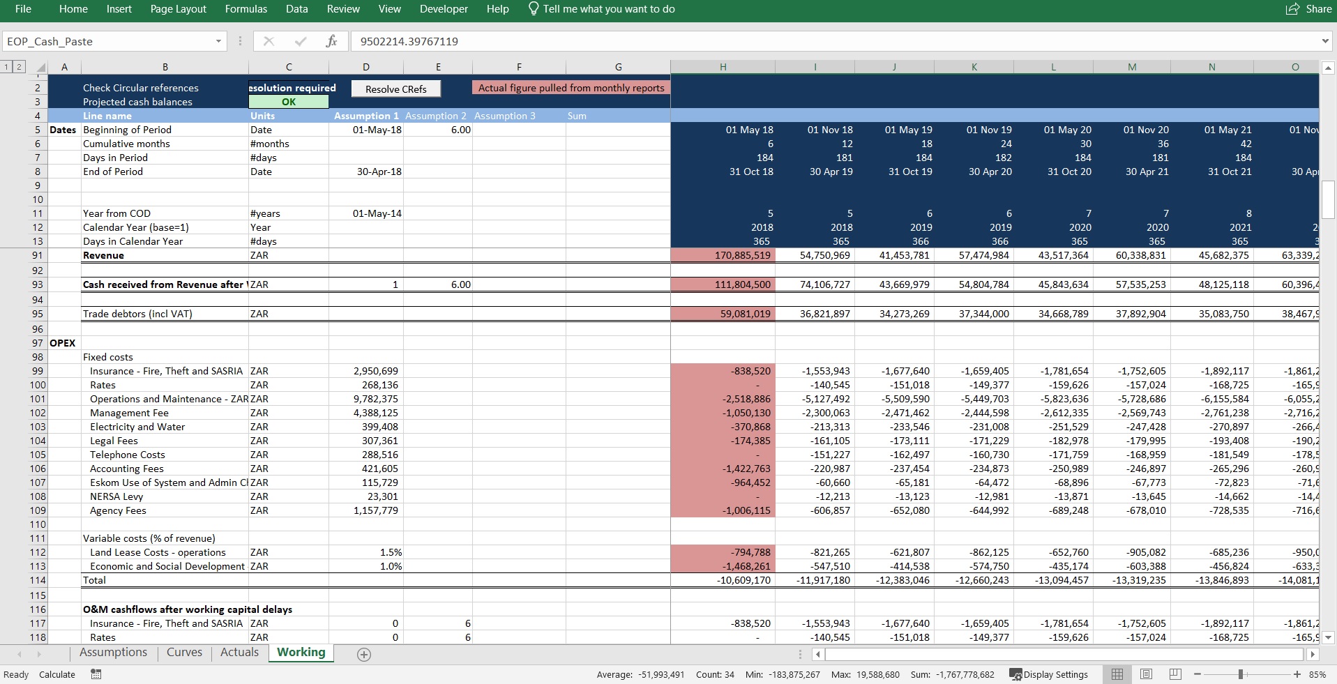
3) The generic project model should be in a single sheet, to the extent possible. By selecting the project in the Assumptions sheet, the calculations will update to represent that project. Given that projects may be structured differently, it may be necessary to have some functionality which is superfluous to some projects, but necessary in others. Examples of this may include multiple debt facilities, a mezzanine facility, O&M bonuses which are structured in a particular fashion, different lease arrangements, and so on. It is necessary that you be able to zero each of these without breaking the model.

4) I created functionality to pull time-based tariffs and balance sheet items into the model. This is because as these change over time, the future distributions to capital providers change too. For example, an increase in tariff (relative to the original base case) will increase the distributions to shareholders. Similarly, a change in the tax depreciation schedule will influence the amount of tax paid in the future and therefore CFADS. It is important that these be included only in the time-based assumptions, and that no changes are made in the calculation sheet, since we will iterate through the projects when working at a portfolio level, and hard-coded figures in the working will clearly break this functionality. You can see an example of these in the Curves sheet in the image above.
5) Now that we have a full project model which is able to represent multiple different project by changing only the assumptions, and the ability to switch between different projects by selecting which set of assumptions to use, it is possible to iterate through the projects using a macro by selecting the relevant project, resolving any circular references, and hard-copying the desired output into a portfolio view for each project. Since each project can have different length and starting-month periods, I used a monthly timeline and a lookup to copy distributions to shareholders (the output I chose for my proof of concept) into a table.

I also created basic error checking, focusing on whether the circular references had been resolved in each iteration, and whether the assumptions in the relevant project were different at the time of running the portfolio consolidation macro to those presently persisting in the model assumptions, using a checksum of the model assumptions.
6) Finally, I aggregated these results into more usable time periods (eg annual), and calculated a range of NPVs.

The approach described here has a few significant advantages:
- Most obviously, the investor only has to understand and maintain a single model.
- This also means that the single model can be audited at much lower cost than auditing several models.
- Implementing scenarios across all projects simultaneously is trivial – for example if the house view on CPI changes, or the VAT rate changes.
- Implementing structural layers, such as structurally-subordinated funding, is also fairly trivial.
Overall, these amount to a significant decrease in the amount of time required to perform any function requiring the project model(s), better operational risk management, reduced costs, and to better understanding of the portfolio.