

The premise for the long/short stock pair arbitrage trade
The long/short stock pair trade is a well-known arbitrage trade, which works as follows:
- Identify two highly-correlated and co-integrated stocks.
- Establish that each stock and the long-short combination of the two stocks is indeed stationary. Steps 1 and 2 are referred to as the Engle and Granger procedure.
- When the two stocks move away from each other, short the stock that has increased in value and go long on the stock that has decreased in value.
- Since the two stocks are highly correlated, they should move back towards each other at some point, closing the gap between them.
- When they do, close out the positions. At this point, the aggregate value of the long/short pair should be greater than zero, since in order for the gap to have closed, the shorted stock should have decreased in value relative to the value of the long stock (or visa versa).
- Since this is a statistical arbitrage strategy, repeat this exercise over as many pairs as is reasonable in order to reduce the possibility of a (hopefully!) low-probability event that the correlation observed to date is simply a statistical fluke which does not continue into the future.
If the premise upon which the trade is based is correct, and the correlated stocks are chosen appropriately, the portfolio should be profitable.
Building the model
I built a model to test this trade based on the more liquid stocks on the Johannesburg Stock Exchange (JSE). Doing so entailed the following steps:
Obtaining stock data:
I downloaded stock data from google finance using excel and vba macros as laid out by Edward Bodmer in his excellent financial model resource website, https://edbodmer.wikispaces.com. To do so, I looped through a list of JSE stockcodes and used the Workbooks.Open (URL) Excel method, where URL is replaced by the URL of the google finance page for the stock I wanted to download. I pushed all of these values into a SQL Server Express database so I could slice and dice the data later when I needed it. Unfortunately google finance doesn’t do adjusted prices (i.e. prices adjusted for share splits and dividends) so this might be a possible augmentation for a later date.
Testing for stationary time series
I filtered my stock data to ensure I only used liquid stocks. Then I generated a list of stock pairs for every combination of liquid stocks. I did this in SQL, before moving each pair into a Python scripting environment where I tested that the change in price of each stock (i.e. ClosePrice today – ClosePrice yesterday) was stationary. To test that each of these two time series was stationary, I used the Augmented Dickey Fuller test, which is available in the statsmodels python module. I used a 95% probability threshold in my test, rejecting any stocks or pairs which were not stationary with probability of at least 95%. These tests were undertaken on roughly a year’s worth of data (October 2015 – October 2016).
Checking for correlation and co-integration
I randomly split the data for for those stocks which had passed the stationarity test (stationarity is actually a real word!) into an 80% training population and a 20% testing population and used this to conduct a regression on the stock pair, with one stock being the input (x) value and the other the output (y) value. Again, I used python, using the LinearRegression model in sklearn. I validated the regression using the remaining 20% of the data, saving the accuracy score and the regression coefficients. For example, SBK = 1872.5c + 0.21 * FSR. (A Standard Bank share will cost you roughly R18.72 + 21% of the price of a FirstRand share).
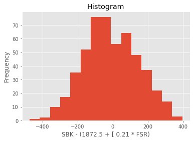
I then generated the modelled prices for the output (y) stock using the data for the training year, subtracted that from the price of the input stock (x) (there’s the long and the short!), and tested the difference for stationarity. If it wasn’t stationary, then, assuming the premise for the pairs trade holds, we couldn’t expect the pair to revert towards each other after they move apart. If it was stationary, then a histogram of the values of the long-short pair (ie the difference) should be approximately normally distributed.
At this point, I had a list of stock pairs that passed the three stationarity tests, a set of regression coefficients describing their relationship, and a measure of how well the regression worked (the accuracy score). I also calculated the standard deviation of the long-short pair, for later use.
I ordered my list of pairs by the regression accuracy, moved my data on a year, and simulated a set of trades.
Simulating trades
To simulate the trades, I started at the beginning of my new year and examined the price of the long-short pair (SBK – [1872.5c + 0.21 * FSR] for my example pair above) for each day moving into the future. If the stocks were perfectly correlated, then they would never move apart and the long-short price would remain at zero. If however, in keeping with the trade’s premise, the shares started to deviate in price (hopefully temporarily!) then the long-short price would move up or down.
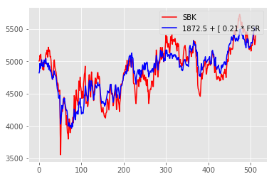
Correlation graph between SBK and FSR: The first half of the graph shows the period over which the correlation model was trained, and consequently fits really well. The second half is the ‘testing’ period, which shows how well the correlation continues into the future.
I chose the following four rules to generate trades for each stock pair (using our SBK-FSR pair as an example):
- Start with a notional cash balance of, say R100,000 (notional because we’re going both long and short… and because it’s fictitious at this point!)
- If the long-short price is above 1 standard deviation, and we’re not already long FSR, then SBK’s price has moved up a lot relative to FSR, so go long on FSR and short on SBK. Go long/short the same amount of R100,000, or whatever balance we have if this isn’t the very first trade.
- If the long-short price is below 0.3 standard deviations and we’re long, then close out the long/short positions. (I.e. move to cash; add the profit or loss to the new notional cash balance)
- If the long-short price is below -1 standard deviation,s and we’re not already short FSR, then SBK’s price has moved down a lot relative to FSR, so go short on FSR and long on SBK. Go long/short the same amount of R100,000, or whatever balance we have if this isn’t the very first trade.
- If the long-short price is above 0.3 standard deviations and we’re short, then close out the long/short positions. (I.e. move to cash; add the profit or loss to the new notional cash balance)
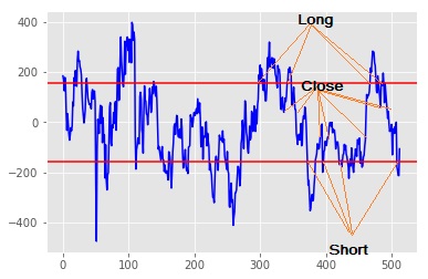
A graph of the daily value of the SBK-FSR long short pair (blue) and a single standard deviation of the values (red). The different trades are indicated by the orange lines: Long = 2 above, Short = 4 and Close = 3 and 5. Recall that trading only starts mid way through the graph.
Repeat this across the full year, and for all the stock pairs.
Finally, check the portfolio value relative to the money put in at the beginning.
Did it work?
I got mixed results. If all the pairs had behaved like the SBK-FSR pair then the trade would have done very nicely. However, they didn’t. Here’re the graphs for the Sibanye Gold, Harmony Gold pair:
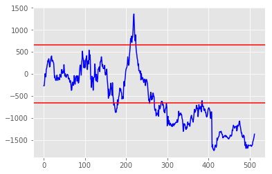
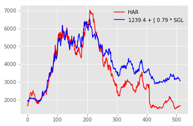
At the start of the trading period (around day 250) this pair looked very feasible. The graphs correlate nicely over the training period and the big swing and reverse around day 180 looks enticing! So let’s trade…
For this pair, we would have shorted Sibanye and bought Harmony around day 260… and we would have continued to hold Sibanye until the end of the trading period, by which time we would be about 10% down, excluding trading and holding costs.
I see your model and I raise you reality
But why? The correlation looked great, and the trade looked so promising. Simply put, circumstances trumped the correlation:

Google search for Sibanye Gold, limited to the last year (and this is the one we shorted!). Harmony Gold’s looks pretty bad too, with illegal mining, strikes, deaths at the mine and managers being murdered.
Consequently, it looks like you need to be a little bit lucky, or apply a little more than statistical determinants to choosing your stock pairs. This is in agreement with the literature, which speaks to “selecting stocks which have a reason to be correlated”. I.e some judgement is required. It also makes sense in a South African context, since our economy feels fragile and prone to shocks right now.
Consequently, an exercise like the one above might be a good starting point for building a pairs trade, but requires both judgement and quite a bit of model tuning.
Afterthoughts:
Any comments or questions are very welcome.
I can think of quite a few model improvements, amongst them:
- A rolling evaluation over the trading period, using data that is in the past, as at the date of trade (rather than a year stale by the end of the trading period)
- Stop losses
- Inclusion of fundamental economic inputs to identify possible reasons for changes in the correlation
- Portfolio constraints, such as exposure limits
- Incorporating price adjustments for stock splits and dividends
- Use of more granular data